G rect - Une boite à outils Matlab pour géoréférencer des images

Introduction

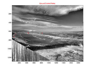
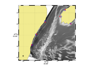
This toolbox contains a series of Matlab functions for georectifying highly oblique digital images. This is useful in oceanography for obtaining quantitative information on sea-surface patterns such as those induced by internal waves, fronts or sea-ice.

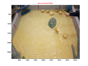
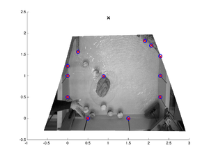
Although this toobox was initially developed to georectify geophysical images it can be used just as well for rectifying laboratory images. The following images show examples of such image rectifications.

Example of a geophysical photo showing sea-ice distribution in the St. Lawrence Estuary.

Same as previous photo once georectified.

Example of a laboratory basin photo.

Same as previous once georectified.

How to get the package

svn co http://bourda02@demeter.uqar.ca/svn/g_rect/trunk

How to use the package

Once expanded the g_rect package is organized as follow:

• g_rect_package
  • src (the source codes)
    • g_rect (contains the mains georectification functions)
    • g_calib (contains camera calibration functions)
    • g_stabilize (contains image stabilization functions)
  • Examples
    • Field (a field example)
    • Lab (a lab example)

The main georectification functions are found within the g_rect directory. The other two directories are for more advanced processing if the camera needs to be calibrated (g_calib) or if you need to stabilize (i.e. removing small movements between successive images) a series of images (g_stabilize). You may not need to play at all with these.

For a quick start let's only play with the main function called g_rect.m found under the g_rect directory. First you should set this directory into your Matlab path (File -> Set Path).

Then go with Matlab into the directory Examples/Field. You will find there an image (IMG_6614.JPG) and a file named parameters.dat. This is the main input parameter file that you need to edit for a given image or for a given series of images.

This input parameter file looks like this:

% I/O information
imgFname = 'IMG_6614.JPG';
firstImgFname = 'IMG_6614.JPG';
lastImgFname = 'IMG_6614.JPG';
outputFname = 'g_rect.mat';

% Field or lab case situation.
% Set field = true for field situation and field = false for lab situation.
field = true;

% Camera position
% lat/lon for field situation
% meter for lab situation
LON0 = -70.6010167;
LAT0 = 47.2713000;

% Offset from center of the principal point (generally zero)
ic = 0;
jc = 0;

% Parameters
hfov = 45.0; % Field of view of the camera
lambda = 2; % Dip angle above vertical (e.g. straight down = 90, horizontal = 0)
phi = 0.0; % Tilt angle (generally close to 0).
H = 720; % Camera altitude
theta = 70.0; % View angle clockwise from North (e.g. straight East = 90)

% Uncertainty in parameters. Set the uncertainty to 0.0 for fixed parameters.
dhfov = 20.0;
dlambda = 10.0;
dphi = 5.0;
dH = 0.0;
dtheta = 20.0;

% Order of the polynomial correction (0, 1 or 2)
polyOrder = 1;

% To save memory calculation can be done in single precision.
% For higher precision set the variable 'precision' to 'double';
precision = 'double';

% Ground Control Points (GCP).
% The data must come right after the gcpData = true
gcpData = true;

360  829  -70.561367  47.303783 

 54  719  -70.54500   47.335 

 99  661  -70.505     47.375 

452  641  -70.435     47.389 

429  633  -70.418     47.408 

816  644  -70.393     47.368 

References

• Bourgault (2008), Shore-based photogrammetry of river ice, Canadian Journal of Civil Engineering Media:Bourgault_2008.pdf.
• Bourgault et al (2011), Field observations of a large-amplitude internal wavetrain and its reflection off a steep slope, Journal of Physical Oceanography Media:Bourgault_et_al_2011a.pdf .
• Farid and Woodward (2007), Video stabilization and enhancement, Unpublished Media:Farid_Woodward_2007.pdf .
• Pawlowicz (2003), Quantitative visualization of geophysical flows using low-cost oblique digital time-lapse imaging, IEEE Journal of Oceanic Engineering Media:Pawlowicz_2003.pdf.