Difference between revisions of "A Matlab package for georectifying oblique digital images (g rect)"
| Line 76: | Line 76: | ||
jc = 0; | jc = 0; | ||
| − | % | + | % Camera parameters |
hfov = 45.0; % Field of view of the camera | hfov = 45.0; % Field of view of the camera | ||
lambda = 2; % Dip angle above vertical (e.g. straight down = 90, horizontal = 0) | lambda = 2; % Dip angle above vertical (e.g. straight down = 90, horizontal = 0) | ||
| Line 83: | Line 83: | ||
theta = 70.0; % View angle clockwise from North (e.g. straight East = 90) | theta = 70.0; % View angle clockwise from North (e.g. straight East = 90) | ||
| − | % Uncertainty in parameters. Set the uncertainty to 0.0 for fixed parameters. | + | % Uncertainty in camera parameters. Set the uncertainty to 0.0 for fixed parameters. |
dhfov = 20.0; | dhfov = 20.0; | ||
dlambda = 10.0; | dlambda = 10.0; | ||
| Line 91: | Line 91: | ||
% Order of the polynomial correction (0, 1 or 2) | % Order of the polynomial correction (0, 1 or 2) | ||
| − | polyOrder = | + | % Be careful with this option as this provides a purely empirical fit not based on any geometrical |
| + | % grounds. Always make first tests with polyOrder = 0, i.e. without any polynomial correction. You | ||
| + | % can then try this correction for a final touch to correct for some unknown errors or distortions. | ||
| + | polyOrder = 0; | ||
% To save memory, calculation can be done in single precision. | % To save memory, calculation can be done in single precision. | ||
Revision as of 17:41, 7 May 2020
Contents
Introduction
This toolbox contains Matlab functions for georectifying highly oblique images. This is useful in oceanography for obtaining quantitative information on sea-surface patterns such as those induced by surface waves, internal waves, fronts, slicks, sea-ice, etc.
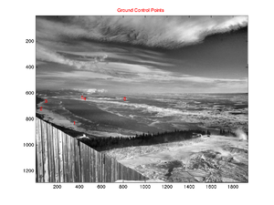
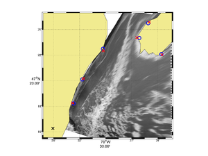
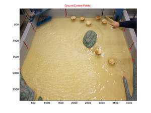
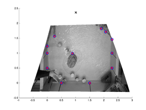
Although this toobox was initially developed for the georectification of geophysical images it can be used just as well for rectifying laboratory images. The following images show examples of such image rectifications.
How to get the package
There are 2 options to get the g_rect package.
- You can download a zipped file that contain the code by clicking on 'Download zip' at the top right corner of the following link: https://gitlasso.uqar.ca/bourda02/g_rect
- You can clone the package either using the https or the ssh protocol. In a terminal window, cd to the directory where you want your code to reside. Then type one of the following two commands at the prompt:
- > git clone https://gitlasso.uqar.ca/bourda02/g_rect.git
- > git clone git@gitlasso.uqar.ca:bourda02/g_rect.git
To update the code to the latest version, simply type the following command from the g_rect top directory:
- > git pull
Once expanded the g_rect package is organized as follow:
- g_rect
- src (the source codes)
- g_rect (contains the main georectification functions)
- g_calib (contains camera calibration functions)
- g_stabilize (contains image stabilization functions)
- utilities
- uwit (functions that may be useful for image equalization)
- DNG2jpg (function to convert raw .DNG images to .jpg images)
- geotiffwrite_20121203 (function to write geotif images)
- m_map (the m_map package)
- src (the source codes)
- Examples
- Field (a field example)
- Lab (a lab example)
The main georectification functions are found within the g_rect directory. The other two directories are for more advanced processing if the camera needs to be calibrated (g_calib) or if you need to stabilize (i.e. remove small camera movements between successive images) a series of images (g_stabilize). You may not need to play at all with these.
g_rect: Quick Start
For a quick start let's only play with the main function called g_rect.m found under the src/g_rect/ directory. Firstly, you should set the entire src/ directory and its subdirectories into your Matlab path (find the Set Path option in the Matlab menu).
Then go with Matlab into the directory Examples/Field. You will find there an image (IMG_6614.JPG) and a file named parameters.dat. This is the main input parameter file that you need to edit for a given image or for a given series of images.
This input parameter file looks like this:
Input file: parameters.dat
% I/O information
imgFname      =  'IMG_6614.JPG';   % This is the reference image
firstImgFname =  'IMG_6614.JPG';   % The first image of a sequence to which the rectification applies.
lastImgFname  =  'IMG_6614.JPG';   % The last image of a sequence.
outputFname   =  'g_rect.mat';     % This is the output filename where the new coordinates will be stored.

% Field or lab case situation.
% Set field = true for field situation and field = false for lab situation.
% Lab situation does not expect to work with latitude and longitude but simply with meters.
field = true;

% Camera position
%   lat/lon for field situation
%   meters for lab situation
LON0 = -70.6010167;
LAT0 =  47.2713000;

% Offset from center of the principal point (generally zero)
ic = 0;
jc = 0;

% Camera parameters
hfov =      45.0;     % Field of view of the camera
lambda =    2;        % Dip angle above vertical (e.g. straight down = 90, horizontal = 0)
phi =       0.0;      % Tilt angle (generally close to 0)
H =         720;      % Camera altitude
theta =     70.0;     % View angle clockwise from North (e.g. straight East = 90)

% Uncertainty in camera parameters. Set the uncertainty to 0.0 for fixed parameters.
dhfov =     20.0;
dlambda =   10.0;
dphi =      5.0;
dH =        0.0;
dtheta =    20.0;

% Order of the polynomial correction (0, 1 or 2)
% Be careful with this option as this provides a purely empirical fit not based on any geometrical
% grounds. Always make first tests with polyOrder = 0, i.e. without any polynomial correction. You
% can then try this correction for a final touch to correct for some unknown errors or distortions.
polyOrder = 0;

% To save memory, calculation can be done in single precision.
% For higher precision set the variable 'precision' to 'double'.
precision = 'double';

% Ground Control Points (GCP).
% The data must come right after the gcpData = true
% Column 1: horizontal image index of the GCP
% Column 2: vertical image index of the GCP
% Column 3: longitude of the GCP (or x-position for lab cases)
% Column 4: latitude of the GCP (or y-position for lab cases)
% Column 5: elevation (in m) of the GCP. Set elevation to 0 if GCP are at water level.
gcpData = true;
360  829  -70.561367  47.303  0
 54  719  -70.54500   47.335  0
 99  661  -70.505     47.375  0
452  641  -70.435     47.389  0
429  633  -70.418     47.408  0
816  644  -70.393     47.368  0
This file contains all parameters required to perform a georectification. You can add spaces and comments as you wish within this file. One specific format however needs to be respected. The ground control points (gcp) must appear right after the variable gcpData = true. These ground control points represent the lon-lat positions associated with some image coordinates.
If you know perfectly some of the camera parameters (e.g. the field of view) you simply have to set the uncertainty of this parameter to zero (e.g. dfov = 0). The algorithm will use precisely this value. Otherwise, for other parameters with some uncertainties, the minimization algorithm will search within the given uncertainty range to find the parameter values that give a best fit between the image control points once georectified and the ground control points (see Bourgault, 2008, for details).
To run the georectification, all you have to do in principle is to edit this parameter file and to type g_rect at the Matlab command line. You will then be prompted for the name of the input parameter file (it does not have to be called parameters.dat). You image will appear with the GCPs as well as a table re-listing all of your parameters. The function will ask you if you're ok with these parameters. If so type enter.
You will then see the algorithm searching the parameter space and will eventually return the result for the set of parameters found. A file will be created, named accoring to the name given in the variable outputFname. This is the main result file that contain all important variables. The most important matrices created are named LAT and LON. These two matrices have the same size as your original image and provides the latitude and longitude of every associated pixel. You can then make a figure using for example the command pcolor (or m_pcolor if you use the m_map package) with LON and LAT as the arguments for the position and a third argument for the pixel intensity which could simply be the mean of the RGB channel if you want to reduce a color image to a grayscale image. Fancier color representation could also be done but this is up to you.
g_calib
Camera calibration could be done if required. All files needed are found in the g_calib folder. The package comes from this site that you should consult for information on how to perform a camera calibration: http://www.vision.caltech.edu/bouguetj/calib_doc/
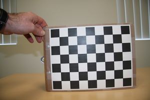
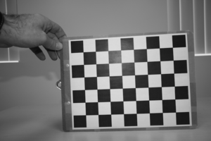
Essentially, a camera calibration removes distortion associated with a lens. The images below shows the effect of such a camera calibration.
Note that this step is not always required for two main reasons. Firstly, it could be that the camera and lens you use has acceptable distortion. Secondly, the algorithm in g_rect provides a polynomial correction (of order 1 or 2) to the image if you have enough ground control points (it is the variable name polyOrder in the input parameter file). This is an indirect way of correcting for lens distortion that might be acceptable, especially if you have ground control points well spread within the image. However, the polynomial correction may be dangerous if your ground control points are clustered within a specific region of the image in which case unrealistic distortions may appear outside the region with ground control points.
g_stablilize
Generally, sequences of images are collected from a fixed tripod. For example, you may want to observe the movement of sea-ice over a semi-diurnal cycle at a sample rate of 1 image per minute (roughly 750 images). If the tripod does not move during the experiment then the georectification procedure described above with g_rect only needs to be applied to one image. The resulting coordinate matrices LAT and LON can then be applied to all images of the sequence.
In practice, the camera may move for many reasons. It may be because you needed to replace the batteries, because you touched the camera by mistake, because you needed to change a camera setting half-way through the experiment or, if you're outside, because wind gusts induced small but perceptible camera movements or if you use a drone. If you don't correct for these movements, the sequence will be jumpy if you make a movie with it. This may lead to inaccurate measurements if you need to compare two frames, say for calculating ice drift velocities (say using PIV) or internal wave phase speeds.
To fix this problem you could apply a new georectification to every images that has moved. This is however not practical if, for example, camera movements were randomly induced by wind gusts. In some windy situations, just about every image show small but perceptible camera movements. You wouldn't want to apply the georectification 100 or thousands of times.
This is when camera stabilization becomes very useful. The idea is to choose one reference image, generally the first image of the sequence, and to geometrically transform all other images, for translation, scale and rotation, to match as close as possible the reference image. This step is done on the normal photos, before doing the georectification.
For this to work properly we need to tell the algorithm which parts of the image are not supposed to have moved. The algorithm cannot tell by itself whether it is the camera that moved or the evolving feature we are documenting (moving ice, evolving fronts or internal wave propagation). These portions of the image that are not supposed to move (e.g. land, islands) are called region of interest (ROI). Details of the stabilizing procedure are described by Farid and Woodward (2007). The Matlab algorithm found in Farid and Woodward (2007) have been adapted here.
The folder g_stabilize contains a series of Matlab functions for performing the image stabilization. However, you need to be familiar with only the following two functions:
g_roi.m
This function is a utility that helps you determine region of interest. To use it you simply have to call the function with your reference image filename such as
g_roi('IMG_1.jpg')
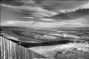
and follow the instructions. Essentially, you will be asked to make polygons around regions of interests (roi). Those are regions in your image that are not supposed to show any movement. Make sure not to include any moving patterns on the water or the sky.
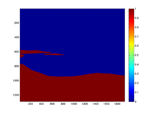
This function only puts 1s in ROIs and 0s everywhere else. Once you're done a file named roi.mat is created. The blue and red image below shows the ROI image corresponding to the image #1. This file is then needed by the next function that performs the actual stabilization.
g_stabilize.m
Once you have created the roi.mat file, copy this file in the folder that contains all images you wish to stabilize and then simply type, in principle, the following command:
g_stabilize(img_ref_fname)
where img_ref_fname is the name (with path and extension) of the reference image against which all images in the current directory will be stabilized against.
For example:
g_stabilize('IMG_2018.jpg')
if the images are in the current directory. Or perhaps
g_stabilize('experiment_1/data/IMG_2018.jpg')
if the images are located somewhere else.
The function will by default create a new directory called 'stable' (unless specified otherwise in the options) in which all images with the same name but with the suffix _stable (by default) will be created. The original images are conserved.
There is a number of options you may want to play with, such has the size of the L-level Gaussian pyramid (default is 4), or whether you want to equalize the image or whether you want to use the gradient of the image for stabilization. In general the stabilization algorithm works really well but it may require some trial and errors and some tweaking for any particular application. Type help g_stabilize to see the available options.
Remark
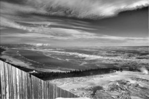
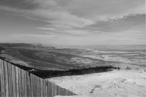
Because of rapidly changing light conditions outside, the stabilize algorithm may not always work as you would hope. This is because region of interests are often subject to moving cloud shadows that may fool the algorithm. In some cases it may be necessary to filter first you image and/or to apply equalizers in order to remove as much as possible such parasite motions. In general, the algorithm does quite a good job but may need some tweaking for some specific applications. You can appreciate the effect by downloading and comparing IMG_1.JPG with IMG_58.JPG and IMG_58_stable.JPG below.
References
Algorithm
- Farid and Woodward (2007), Video stabilization and enhancement, Unpublished.
- Pawlowicz (2003), Quantitative visualization of geophysical flows using low-cost oblique digital time-lapse imaging, IEEE J. Ocean. Eng.
Application examples
- Bourgault, Galbraith and Chavanne (2016), Generation of internal solitary waves by frontally-forced intrusions in geophysical flows, Nat. Commun.
- Bourgault and Kelley (2003), Wave-induced boundary mixing in a partially-mixed estuary, J. Mar. Res..
- Bourgault (2008), Shore-based photogrammetry of river ice, Can. J. Civil Eng..
- Bourgault et al (2011), Field observations of a large-amplitude internal wavetrain and its reflection off a steep slope, J. Phys. Oceanogr.
- Richards et al (2013), Measurements of shoaling internal waves and turbulence in an estuary, J. Geophys. Res.
- Wang and Pawlowicz (2011), Propagation speeds of strongly nonlinear near‐surface internal waves in the Strait of Georgia, J. Geophys. Res.
- Wang and Pawlowicz (2012), Oblique wave-wave interactions of nonlinear near-surface internal waves in the Strait of Georgia, J. Geophys. Res.
Contributing authors
- Daniel Bourgault - Institut des sciences de la mer de Rimouski (email: daniel_bourgault@uqar.ca)
- Clark Richards - Woods Hole Oceanographic Institution (email: clark.richards@dfo-mpo.gc.ca)
- Rich Pawlowicz - University of British Columbia (email: rich@eos.ubc.ca)
